The degree of flatness or peakedness is measured by kurtosis. It tells us about the extent to which the distribution is flat or peak vis-a-vis the normal curve. Diagrammatically, shows the shape of three different types of curves.

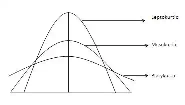
The normal curve is called Mesokurtic curve. If the curve of a distribution is more peaked than a normal or mesokurtic curve then it is referred to as a Leptokurtic curve. If a curve is less peaked than a normal curve, it is called as a platykurtic curve. Kurtosis is measured by moments and is given by the following formula:

Formula

β2=μ4μ2β2=μ4μ2

Where −

·        μ4=∑(x−x¯)4Nμ4=∑(x−x¯)4N

The greater the value of \beta_2 the more peaked or leptokurtic the curve. A normal curve has a value of 3, a leptokurtic has \beta_2 greater than 3 and platykurtic has \beta_2 less then 3.

Example

Problem Statement:

The data on daily wages of 45 workers of a factory are given. Compute \beta_1 and \beta_2 using moment about the mean. Comment on the results.

Wages(Rs.)	Number of Workers
100-200	1
120-200	2
140-200	6
160-200	20
180-200	11
200-200	3
220-200	2

Solution:

Wages (Rs.)	Number of Workers (f)	Mid-pt m	m-1702017020 d	fdfd	fd2fd2	fd3fd3	fd4fd4
100-200	1	110	-3	-3	9	-27	81
120-200	2	130	-2	-4	8	-16	32
140-200	6	150	-1	-6	6	-6	6
160-200	20	170	0	0	0	0	0
180-200	11	190	1	11	11	11	11
200-200	3	210	2	6	12	24	48
220-200	2	230	3	6	18	54	162
	N=45N=45			∑fd=10∑fd=10	∑fd2=64∑fd2=64	∑fd3=40∑fd3=40	∑fd4=330∑fd4=330

Since the deviations have been taken from an assumed mean, hence we first calculate moments about arbitrary origin and then moments about mean. Moments about arbitrary origin ‘170’

μ11=∑fdN×i=1045×20=4.44μ12=∑fd2N×i2=6445×202=568.88μ13=∑fd2N×i3=4045×203=7111.11μ14=∑fd4N×i4=33045×204=1173333.33μ11=∑fdN×i=1045×20=4.44μ21=∑fd2N×i2=6445×202=568.88μ31=∑fd2N×i3=4045×203=7111.11μ41=∑fd4N×i4=33045×204=1173333.33

Moments about mean

μ2=μ′2−(μ′1)2=568.88−(4.44)2=549.16μ3=μ′3−3(μ′1)(μ′2)+2(μ′1)3=7111.11−(4.44)(568.88)+2(4.44)3=7111.11−7577.48+175.05=−291.32μ4=μ′4−4(μ′1)(μ′3)+6(μ1)2(μ′2)−3(μ′1)4=1173333.33−4(4.44)(7111.11)+6(4.44)2(568.88)−3(4.44)4=1173333.33−126293.31+67288.03−1165.87=1113162.18μ2=μ2′−(μ1′)2=568.88−(4.44)2=549.16μ3=μ3′−3(μ1′)(μ2′)+2(μ1′)3=7111.11−(4.44)(568.88)+2(4.44)3=7111.11−7577.48+175.05=−291.32μ4=μ4′−4(μ1′)(μ3′)+6(μ1)2(μ2′)−3(μ1′)4=1173333.33−4(4.44)(7111.11)+6(4.44)2(568.88)−3(4.44)4=1173333.33−126293.31+67288.03−1165.87=1113162.18

From the value of movement about mean, we can now calculate β1β1 and β2β2:

β1=μ23=(−291.32)2(549.16)3=0.00051β2=μ4(μ2)2=1113162.18(546.16)2=3.69β1=μ32=(−291.32)2(549.16)3=0.00051β2=μ4(μ2)2=1113162.18(546.16)2=3.69

From the above calculations, it can be concluded that β1β1, which measures skewness is almost zero, thereby indicating that the distribution is almost symmetrical. β2β2 Which measures kurtosis, has a value greater than 3, thus implying that the distribution is leptokurtic.