As we have seen in Chapter 4, failure rate often changes with time (Fig. 1 there). This is because the main causes of failures change with time. The early failures (stage I) are mostly caused by errors in design, manufacture, assembly, or building process or due to hidden defects, and the instant of their occurrence cannot be predicted. The failures in stage II (useful life) arise from external reasons (random overloading, collision with another object, climatic events, and errors of personnel) and also cannot be predicted. Only if the pertinent failure rate is known one can predict approximately how often failures can be expected and take suitable measures to mitigate their effects. The failures in stage III (aging and wear-out) arise due to the internal “weakness” of the object and appear after some time of operation even under appropriate conditions of use. Many objects fail due to wear, fatigue, creep, corrosion, or other processes of gradual deterioration. Fortunately, in such cases a possibility exists to predict (with higher or lower accuracy) the time when the object is about to fail, provided that the relationship between the load intensity and the rate of deterioration is known.
Two principal ways exist:
1. If the basic mechanism of degradation is known, one can express the deterioration rate as a function of the characteristic load and then derive a formula for the calculation of the time to failure. For the known load, the time to failure can thus be predicted in advance (e.g. during the design stage). Vice versa, it is possible to find such dimensions of loaded parts, which will guarantee an acceptably low rate of deterioration and thus the demanded life.
2. Due to deterioration, the load response of many objects also gradually changes. If a quantity characterizing the degradation is known (e.g. the magnitude of vibrations), it is possible to monitor its time development in the real object. These data can be extrapolated, and the time can be predicted at which the characteristic quantity reaches the critical value.
Both approaches may be combined. During design, the time to failure can be predicted, and during operation, this prediction is updated with respect to the actual time history of the operation and response. The object is never allowed in operation until the instant of expected failure. At a reasonable time before it, a check of its condition is made and a suitable time for repair or next inspection is proposed. Both cases will be discussed here in detail.
Prediction of the time to fatigue failure from the law of material degradation
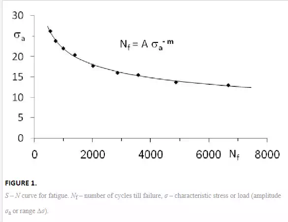
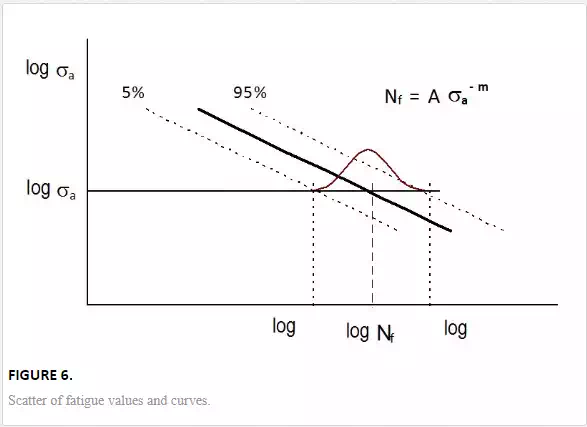
A typical example is the fatigue of metallic parts under cyclic or periodic loading. If the characteristic stress is higher than the so-called fatigue limit, a small crack arises in the component after some time of operation and grows slowly, and when it reaches the critical size, the component breaks. The number of cycles to failure Nf depends on the stress amplitude σa in the loading cycle [1, 2]. In the simplest case, it can be expressed by the so-called S – N (or Wöhler) curve (Fig. 1):
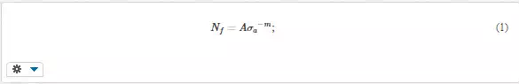
A and m are constants obtained by testing the material or component. Several variants of fatigue equation exist, but, basically, their character is similar to Equation (1). Sometimes, the stress range in the loading cycle, ∆σ = σmax – σmin, is worked with instead of the stress amplitude σa
This formula can be used in the dimensioning of a component for a certain prescribed life.
Time to fatigue failure of objects with cracks
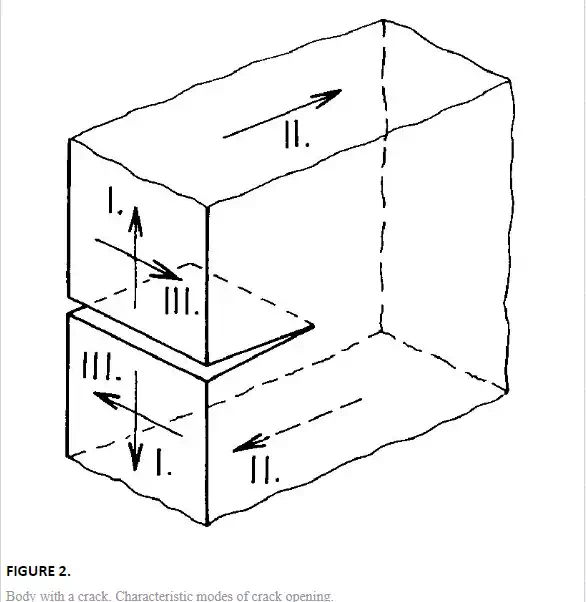
Equation (1) does not assume any previous damage to the component. Sometimes, however, one or more cracks or similar defects are present in the body from the beginning. The behavior of bodies with cracks is studied by fracture mechanics [1 – 4]. Crack growth is influenced not only by the stress, but also by the crack size (Fig. 2). Both quantities form together a very important parameter, called stress intensity factor K,

σ is the nominal stress in the crack region, a is the characteristic length of the crack, and Y(a) is a factor characterizing the crack shape and size and stress distribution. The subscript of K denotes the mode of crack opening; number I means simple opening, which is the most important case. If the stress intensity factor attains the critical value KC for the given material, fast fracture follows. The corresponding critical crack length is

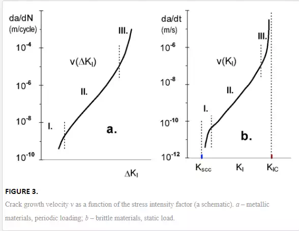
In components exposed to periodic loading, the crack can grow very slowly even if the stress intensity factor is lower than the critical value. The period of subcritical crack growth can last from minutes to years and can be predicted via the relationship between the crack velocity and the stress intensity factor. The crack velocity v during the period most important for delayed failure (region II in Fig. 3a) can often be approximated by the Paris-Erdogan equation [3]:
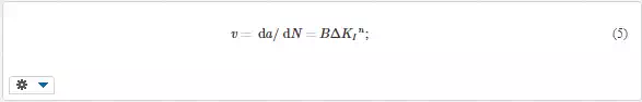
da/dN is the increment of crack length per loading cycle, ∆KI is the range of stress intensity factor in the loading cycle, ∆KI = KI,max – KI,min, and B and n are the constants for the given material and environment. Inserting ∆KI from the modified Equation (3) into Equation (5) and separating a and N, one can arrive at the following expression for the number of cycles for the crack growth from the initial length ai to the length a
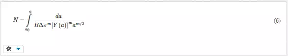
Fast fracture occurs if the stress intensity factor attains critical value KIC, also called fracture toughness. The corresponding critical crack length ac, used as the upper limit in the integral (6), is given by Equation (4), with σmax denoting the maximum stress in the loading cycle. The resultant formula for Nfin the simplest case (constant stress range, small crack enlargement, and thus Y ≈ const) is basically similar to Equation (1), with ∆σ instead of σa. The number of cycles to failure is roughly indirectly proportional to some power of the characteristic stress range or amplitude. It is thus possible in design to propose such dimensions of the cross-section that the stresses will be so low to guarantee the demanded lifetime.
Static fatigue, wear, and creep
In some materials, fatigue occurs even under constant load. Examples are glass and some ceramics as well as some metals in a corrosive environment. In this case, called static fatigue, it is possible to express the time to failure tf as a function of acting stress. The velocity v of very slow crack growth depends not on the amplitude but on the value of the stress intensity factor KI (Fig. 3b), and in the important part of the v(K) diagram, the velocity can be approximated by a power-law function

The relationship for the time to failure is similar to Equation (1) or (6) with the stress amplitude σareplaced by characteristic stress σ and the number of cycles Nf by the time to failure tf. The relationships similar to Equation (1) are also used for the prediction of the life of ball bearings and other components exposed to wear or of parts exposed to creep and other kinds of gradual deterioration. In all these cases, the time to failure is roughly indirectly proportional to some power of the characteristic load P

the time to failure in rotating parts can be expressed by means of a number of revolutions. Equation (8) is the simplest formula; the relationship in some cases is more complex. For details, the reader is referred to a special literature, for example [1 – 4].
The consequences of random variability of load and uncertainties in the determination of parameters in fatigue equation will be dealt with in Chapter 19.
Variable loading
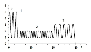
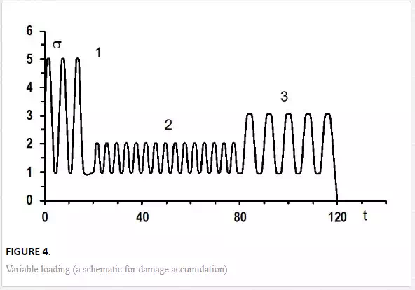
Until now, we have assumed a constant load amplitude. Often, it varies. Figure 4 depicts a regular operation regime of a machine, with four characteristic stages. Examples of irregular or random regime are bogie of a car or components of an engine. In all these cases, the concept of damage accumulationis used. Various hypotheses and models have been proposed [1, 2]. Here, only the simplest concept of linear damage accumulation, also named the Palmgren-Miner rule, will be explained
The basic idea of the Palmgren-Miner rule is that every loading cycle contributes to damage and exhausts a minute part of the life. Damage (in fact relative damage) D is then defined as the ratio of the number of loading cycles, which the object has undergone, and the number of cycles (under the same kind of loading), which would cause failure
For example, if a component could sustain 1000 loading cycles until failure, then one loading cycle has exhausted 1/1000 of its fatigue life. Failure occurs if N = Nf, that is if D = 1 (in this case, D = 1 for N = 1000). Note the difference between N and Nf !
If the loading pattern is more complex, consisting of various loading blocks, each with different amplitude and different number of loading cycles (Fig. 4), the total damage is obtained as the sum of damages caused during the individual blocks,
Again, failure occurs if D = 1. In this way, it is possible to find the number of loading cycles or blocks until failure. If the damage, corresponding to one day of operation, is D1, then the object can sustain 1/D1 days before it fails.
Special procedures have been developed for cases where the load changes irregularly, in a random way, such as constructions of airplanes or cars. For more, see [1 – 3].
Prediction of the time to failure from the response
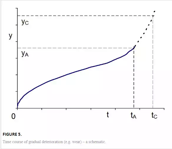
The gradual deterioration of many objects can be characterized by various quantities, such as amplitude of vibrations, noise level, deformation under load, or loss of material by wear or corrosion. The pertinent quantity (y) grows gradually to the critical value, corresponding to failure or just an unacceptable condition (Fig. 5). In some cases, it is possible to monitor this quantity and its development in time. These data can be fitted by a suitable function y(t), and the time to failure is predicted as such, for which y reaches the critical value yC (Fig. 5). The knowledge of yC is thus very important. However, it cannot be predicted accurately due to uncertainties in the determination of material parameters, loads, influence of environment, and other factors. For these reasons, the object may never be let in operation till the instant of expected failure. At a reasonable time before it, a check of its condition must be done. This time is denoted as alert, tA, with the appropriately chosen value yA. The determination of tA is also shown in Figure 5. At this time, the object is inspected, and the obtained value y(tA) serves as a base for the decision on the maintenance, renovation, termination of further operation, or allowing the object in operation until the next inspection. Practical examples are shown at the end of this chapter.
Probabilistic aspects of the deterioration curves and lifetime prediction
When dealing with the constants of a fatigue curve, taken from the material data sheets, or with the constants of a curve showing the development of a certain parameter with time, one must not forget that they are only approximate, obtained by testing several samples only. One should always be aware of the scatter of individual values. Actually, each curve corresponds to a particular specimen despite the same test conditions. The testing of many samples would thus give a group or distribution of S – N or similar curves (Fig. 6). The data can be processed in several ways. It is possible to use all experimental data points and calculate the parameters corresponding to the “average” curve, giving the “mean” times to failure. In this case, however, the actual times to failure will be in 50% of all cases longer than the times calculated using these parameters and in 50% shorter, which could be dangerous. The reliability of the prediction can be increased using confidence band around the regression curve based on the scatter of the individual values around this curve (see also Chapters 18 and 19). Another approach fits only certain quantiles of the times to failure for various stress levels. In this way, for example, the 5% quantile curve can be obtained. This is such curve that the probability of failing earlier is only 5%. Similarly, the curves for other reliabilities can be constructed. This approach is possible if many data points (several tens or more) are available.
When taking the constants for calculations from a material database or literature, one should therefore know how they were obtained and to what conditions they correspond. Scatter also influences the values of other material parameters, such as strength, fracture toughness KIC, constants in the equation for subcritical crack growth or for creep, and so on. Also here, one must distinguish between the work with the mean values or with certain quantiles.
The uncertainty due to the scatter of experimental data must always be considered in the predictions of the time to failure or the alert time. The higher uncertainty, the longer time before reaching the critical state should an inspection be made. We return to this topic in Chapter 19.
Example 1
A component is loaded by the sinusoidal mechanical stress of the amplitude σa = 120 MPa. The fatigue (S – N) curve of the material (cf. Fig. 1) is Nf = Aσa– m, with the constants m = 4.0 and A = 5.0 × 10¹³(for σa given in MPa).
Task. Determine the number of cycles to failure Nf. What part of the life will be exhausted after N = 20,000 loading cycles?
Solution. Nf = Aσa–m = 5.0 × 1013 × 120–4.0 = 241,126 cycles.
D = N / Nf = 20,000 / 24,1126 = 0.0829 = 8.29 %.
Example 2
Determine the allowable stress amplitude for the component from Example 1.6/1 so that the component can sustain N = 600,000 cycles.
Solution. The rearrangement of the S – N curve gives σa = (A/Nf)1/m. With N = 600,000 and the constants m = 4.0 and A = 5.0 × 10¹³, the allowable stress is 5.0 × 10¹³/600,0001/4.0 = 95.54 ≈ 95 MPa.
Note. In reality, some factor of safety would be used, either for increasing the number of cycles to failure or for reducing the allowable stress. The stress can be reduced by more ample dimensioning.
Example 3
The technical condition of a machine can be characterized by the amplitude y of vibrations. This amplitude was measured once a day. During 10 days, the following values were measured:
DayNo.:y(mm):10.10−−20.12−−30.16−−40.20−−50.24−−60.28−−70.33−−80.42−−90.48−−100.62DayNo.:1−2−3−4−5−6−7−8−9−10y(mm):0.10−0.12−0.16−0.20−0.24−0.28−0.33−0.42−0.48−0.62
Task. Fit the measured data: (a) by a straight line, and (b) by exponential function and predict:
1. the amplitude on 14th day, and
2. when the amplitude will reach the critical value yc = 1.00 mm.
Solution. The measured data were plotted using Excel. Then, the command Add Trendline was used (Fig. 7). Linear approximation (a) was: y = a + bt = – 0.002667 + 0.054121t; the coefficient of determination, characterizing the quality of fit was r2 = 0.9445. Exponential fit (b) was y = 0.085250 × exp(0.19762t), with the coefficient of determination r2 = 0.9952. (Remark: The higher the r2, the better fit; r2 = 1 means perfect fit.)
The approximations have given the following amplitudes of vibrations on 14th day: ylin = 0.755 mm according to the linear fit, and yexp = 1.356 mm according to the exponential fit. The amplitude y = 1.00 mm could be expected for t = 18.52 days according to the linear fit and for t = 12.46 days according to the exponential approximation.
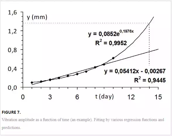
One can see the big differences between the predictions done using different approximations. Caution is necessary especially for longer intervals of predictions and also with respect to the consequences of a wrong prediction