In the next experiment, we ‘turn off’ the waterfall switch. This activates the iterative/incremental gene and the feature-driven gene, such that our project is now broken up into 4 equally sized releases that are delivered in regular intervals in feature sets. Executing the model with these settings produces the following project performance results:
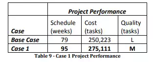
Looking at these results, we find that the same project now takes 16 extra weeks, ending at week 95, and incurs extra cost (roughly 25000 more tasks). However, the product now is delivered with zero defects. Cost and Quality graphs can be observed below in Figure 71.
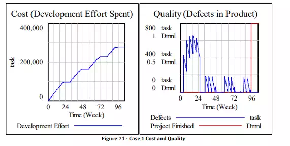
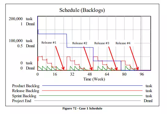
Moreover, there is a much more subtle difference generated by this case: the software is now delivered in four releases, i.e. four functional increments. These are annotated below on the Schedule graph in Figure 72. Each release is not just a random chunk of the software, but a cohesive feature set that is “potentially shippable” and has client/end-user value. Each release can be tested against system-level specifications and user expectations.
This can be of tremendous value to the recipient of the software release: they can immediately start providing feedback and acting as a “beta-tester” as of release #1 in week 24. If the recipient of this release is an integration, test, or quality assurance organization, they can get a head start on testing the software against the system specifications, performing boundary case testes, and so on. In fact, depending on the project environment, being able to several early increments of functionality may be more valuable to the customer than the added cost incurred by this case.
Case 2: Introduction of Micro-Optimization.
Next, we will enable Micro-Optimization. As explained earlier (section 3.3.4), this model element simulates the management policy of empowering the development team to self-manage workload, and to perform process tweaks in between sprints, using learning from prior sprints to improve future sprint performance . We start by setting the Agile Levers for case 2. Running the model with these two genes now produces the following project performance results:
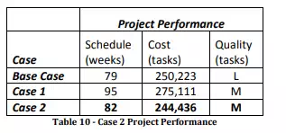
We see improved project duration, down to 82 weeks instead of 95 in case 1. Our costs of around 244K tasks are also lower than both the base case (250K tasks) and case 1 (275K tasks).
Although this may seem counter-intuitive to management, the results here suggest that a team empowered to self-regulate their workload may curtail costs and schedule overrun as opposed to an incremental delivery model whose releases are dictated in advance. Given more time, it is almost always possible to improve the product and this could lead to the “gold-plating” effect where teams spend time over-engineering the product beyond what is necessary to achieve the desired functionality (it is almost the opposite of ‘technical debt’). However, the fact that agile iterations are time-boxed and are feature-driven mitigates this issue, as teams will give priority and focus to completing specific features.
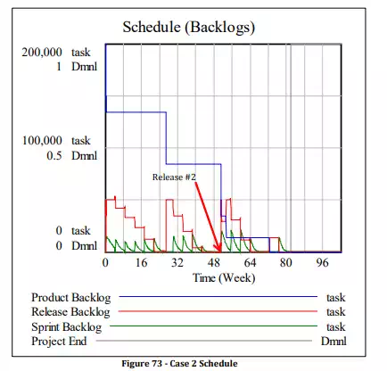
If we examine our work backlogs in Figure 73, we see that roughly two-thirds of the functionality is delivered in the first two releases, around week 50. What has happened here, as opposed to the previous case, is that teams can gradually handle more work than was allotted to them per-sprint in the previous case, and have self-regulated the amount of work they do per-sprint. This allows them to get more sprints completed by week 50 than in the previous case.