Reliability is usually characterized by the probability of failure or by the time to failure. If failure is considered as a single event (e.g. collapse of a bridge), regardless of the time, only its probability is of interest. If we want to know when the failures can occur, their time characteristics are also important. In this chapter, time-dependent failures will be dealt with. Here, one must distinguish between unrepaired and repaired objects depending on whether the failed object is discarded or repaired and again put into service.
Unrepaired objects
The basic quantity for unrepaired objects is the time to failure tf. If a group of identical objects is put into operation, the individual pieces begin to fail after some time, and it is also possible to express the number of failed pieces as a function of time, nf(t). A more universal quantity is the relative proportion of the failed items, that is, the number of the failed items related to the number n of monitored objects, nf(t)/n. This ratio approximately expresses the probability of failure F(t) during the time interval <0; t>;
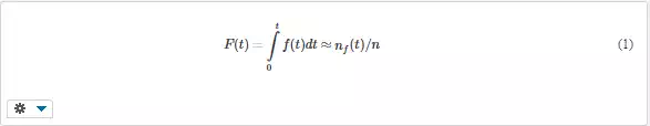
Function F(t) is the distribution function of the time to failure, also called failure function (Fig. 1a). An aid for easier remembering: the letter F is also the first letter of the word failure.
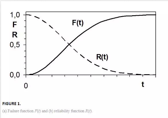
The probability of failure-free operation R(t) expresses the probability that no failure occurs before the time t;
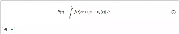
R(t) shows the gradual loss of serviceable objects (Fig. 1b) and is called reliability function (therefore the symbol R). R is complementary to F
The probability density of the time to failure, f(t), expresses the probability of failure during a very short time interval ∆t at time t, related to this interval:
the unit is s-1 or h-1. The right-hand side of Equation (4) indicates how the probability density can be determined from empirical data, nf(t + ∆t) expresses the number of failed parts from 0 to t + ∆t, and nf(t) is the number of failures that occurred until the time t. In fact, probability density f(t) shows the distribution of failures in time, similar to Fig. 3a in Chapter 2. Useful information on reliability is obtained from a very simple characteristic, the average or mean time to failure or MTTF, which is generally defined as
The mean time to failure can be calculated from operational records as the average of the group of measured times to failure,
Remark: Equation (6) is appropriate if all objects have failed. If components with very long life are tested, the tests are usually terminated after some predefined time or after failure of certain fraction of all components. In such cases, modified formulas for MTTF must be used; see Chapter 20 or [1].
Repaired objects
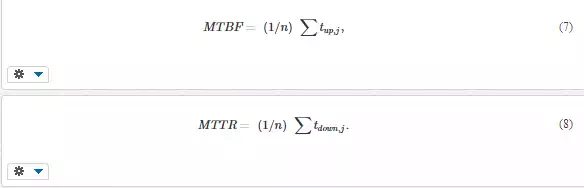
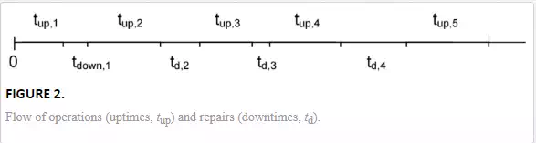
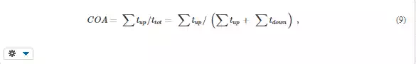
If a repairable item fails, it is repaired and again put into operation. After the next failure, it is again repaired and put into operation, etc. One can thus speak of a flow of operations and repairs (Fig. 2). If we denote each interval as “uptime” tup or “downtime” tdown, we can calculate the mean time between failures, MTBF, and the mean time to repair, MTTR:
If data for a high number of values tup and tdown are available, the distribution of these times can also be obtained and used
. 
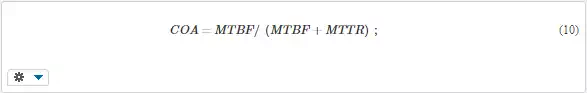
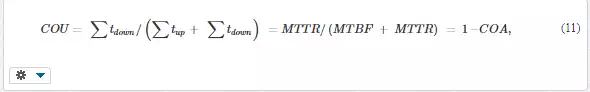
The mean time between failures and mean time to repair can be used to characterize the probability that the object will be serviceable at a certain instant or not. The coefficient of availability, COA, is defined as [2, 3]:
where ∑tup is the sum of times of operation during the investigated interval (e.g. 1 month or year), ∑tdown is the sum of down times in this interval, and ttot is the total investigated time. The coefficient of availability can also be calculated as
MTBF is the mean time (of operation) between failures and MTTR is the mean time to repair (generally, the mean down time caused by failures).
The coefficient of availability simply says what part of the total time is available for useful work. It also expresses the average probability that the object will be able to fulfill the expected task at any instant.
The complementary quantity, coefficient of unavailability
says how many percent of the total time are downtimes. It also expresses the probability that the object will not be able to perform its function at a demanded instant. For example, COA = 0.9 means that, on average, the vehicle (or machine) is only 90% of all time in operation, and 10% of the total time it is idle due to failures. In other words, there is a 90% probability that the object will be available when needed and a 10% probability that it will not be available. Even the simple records from operation can give the basic values of probabilities and reliability.
It must reminded here that the time of a repair is not always the same as the downtime when the object (e.g. a machine) does not work. In addition to the net time of the repair, some logistic times are often necessary, which sometimes last much longer than the repair.
Failure rate
A very important reliability characteristic isfailure rate λ(t). Basically, failure rate expresses the probability of failure during a time unit. Unlike probability, which is nondimensional, failure rate has a dimension. It is t-1, for example, h-1 or % per hour for machines, components, or appliances, km-1 for vehicles, etc. Two cases must be distinguished, depending on whether the object after failure is repaired or not.
Unrepaired objects
The failed item is discarded. This is typical of simple unrepairable objects, such as lamp bulbs, screws, windows, integrated circuits, and many inexpensive parts. Also, a living being cannot be repaired, if it has died. Some objects could be repaired after failure but are not, because of economic reasons. Thus, the term nonrepaired objects can be used as more universal. Failure rate expresses the probability of failure during a time unit but is related only to those objects that have remained in operation until the time t, that is, those that have not failed before the time t. Failure rate is defined as
f(t) is the probability density of failure (=dF/dt), and R(t) is the probability that the object was operated until the time t. An illustrative idea of failure rate can be gained from a simple formula for its calculation from the data from operation:

n is the total number of the monitored objects, nf(t) is the number of the objects failed until the time t, [nf(t + ∆t) – nf(t)] is the number of objects failed during the time from t to t + ∆t, and ∆t is a short time interval. [Remark: Formula (13) is only approximate and often exhibits big scatter. A more accurate value of the instantaneous failure rate λ(t) can be obtained from several nf values occurring in a wider interval around the time t.] The fraction of failed objects, F(t), increases with time, and the fraction of objects that have not failed, R(t), decreases. Equation (1) relates mutually three variables: λ, f, and R. Fortunately, it can be transformed into simple relationships of two quantities. First, it can be rewritten as follows:

The separation of the variables leads to the differential equation of first order,

The integration and transformation lead to the following expression for the probability of operation as a function of time:

The probability of failure is
With respect to Equations (12) to (17), any of the four quantities f, F, R, and λ is sufficient for the determination of any of the remaining three quantities.
The mean time to failure can be calculated using Equation (5).
Repaired objects
After a failure, the object is repaired and continues working. In complex systems, the failed part can also be replaced by a good one to reduce the downtime. The number of working objects remains constant, so that R(t) = 1. Failure rate (1) thus corresponds to the failure probability density, λ(t) = f(t). In this case, the term hazard rate is used as more appropriate, but the expression failure rate is also very common.
Example 1
The monitoring of operation and repairs of a certain machine has given the following durations of operations and repairs: tup,1 = 28 h, tdown,1 = 3 h, tup,2 = 16 h, tdown,2 = 2 h, tup,3 = 20 h, tdown,3 = 1 h, tup,4 = 10 h, tdown,4 = 3 h, tup,5 = 30 h, and tdown,5 = 2 h.
Tasks.
1. Determine the mean time between failures and mean time to repair.
2. Determine the coefficient of availability (COA) and unavailability (COU).
3. Express the average probability (in %) that the machine (a) will be able to work at any instant (R) and (b) will not be able to work (F).
Solution
1. Mean time between failures MTBF = ∑tup,j/n = (28 + 16 + 20 + 10 + 30)/5 = 104/5 = 20.8 h. Mean time to repair MTTR = ∑tdown,j/n = (3 + 2 + 1 + 3 + 2)/5 = 11/5 = 2.2 h.
2. Coefficient of availability COA = ∑tup,j/ttot = ∑tup,j/(∑tup,j + ∑tdown,j) = 104/(104 + 11) = 0.90435. Coefficient of unavailability: COU = ∑tdown,j/ttot = 11/(104 + 11) = 0.09565. Another way of calculation: COA = MTBF/(MTBF + MTTR) = 20.8/(20.8 + 2.2) = 0.90435 and COU = MTTR/(MTBF + MTTR) = 2.2/(20.8 + 2.2) = 0.09565.
3. The probability that the machine will be able to work at any instant equals the coefficient of availability; R = COA = 0.90435 ≈ 90,4%. Similarly, F = COU = 0.09565 ≈ 9.6%.
Example 2
In a town, N = 30 buses are necessary for assuring reliable traffic on 15 routes. However, due to failures and maintenance, several buses are unavailable every day. As it follows from long-term records, the mean availability of the buses is COA = 0.85. How many reserve buses (Nr) are necessary? What is the total necessary number of buses Ntot?
Solution
The coefficient of availability can be calculated as the number of operable buses, Nup, divided by the total number of vehicles, COA = Nup/Ntot, from which Ntot = Nup/COA. With the above numbers, Ntot = 30/0.85 = 35.29. To reliably ensure the public traffic, 36 buses are thus necessary. The number of reserve vehicles is 36 – 30 = 6 buses.
buses are thus necessary. The number of reserve vehicles is 36 – 30 = 6 buses.