In this case we will allow refactoring. As described earlier (5.2.3) this means that when the “technical/design debt” for the project reaches a threshold, the development team will take time to work on additional refactoring tasks to improve the quality of the software and keep it flexible and easy/cheap for expansion and addition of future features.

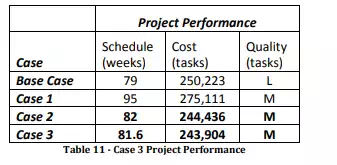
Executing the model thus, with three of the genes, now produces the following project performance results:

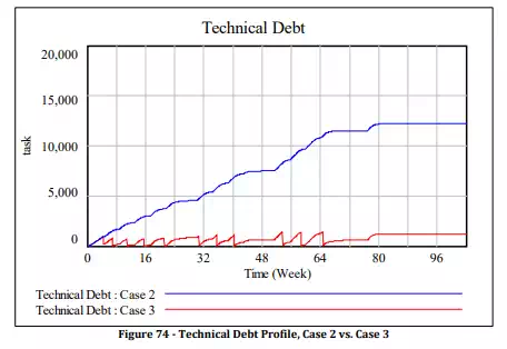
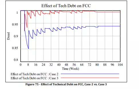
Intuitively, management may have thought that allowing refactoring is akin to scope creep, and thus may have thought that this would have increased either our cost or slipped the schedule. Our results, on the contrary, show that allowing refactoring resulted in a very minor (albeit negligible) improvement in schedule and in cost. To explain this, let us take a look at the graph for Technical Debt in case 3 vs. case 2 – see Figure 74. As can be observed in this graph, refactoring keeps our technical debt’s “balance” low by refactoring. This is turn has a less detrimental effect on our Fraction Correct and Complete than when letting technical debt get out of hand, as shown in Figure 75.

Finally, there is one more subtle benefit observed in this case. Since we are now delivering the software in multiple releases, let’s look at the number of undiscovered rework tasks in the software at each release. This is shown in Figure 76.

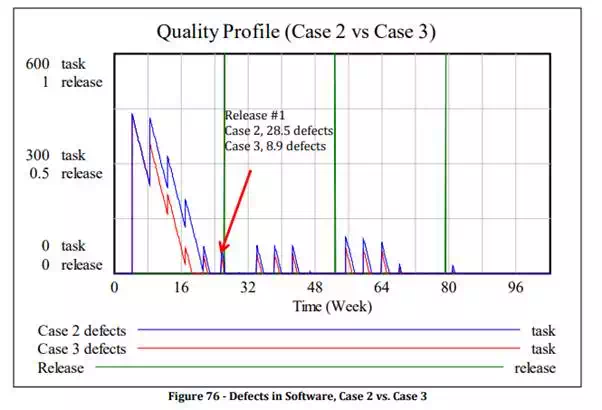
Here we find that in case 2, the software was released with 28.5 defects, vs 8.9 defects in case 3 where refactoring was allowed. In other words, refactoring also allows the development team to produce better quality incremental releases. This makes sense intuitively, as it is clear that refactoring to optimize will improve the quality of the software, however the surprising part is the previous finding: that refactoring has no detrimental effect on cost or schedule. This is because of the positive effect that unpaid technical debt has on defect generation.

Case 4: Introduction of Continuous Integration

We now activate the Continuous Integration lever. This will create an initial load in tasks to be performed, representing the initial effort to set up and configure the development and delivery environment. Later, once that environment is available, it enhances productivity, and our ability to detect rework tasks (thanks to automated testing).

Executing the model with these parameters produces the following project performance results:

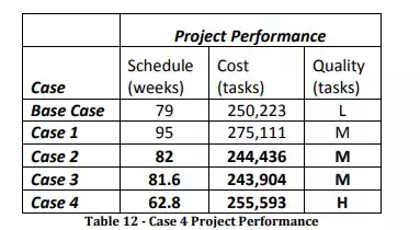
There are no surprises here: Introducing Continuous Integration increases cost somewhat, due to the up-front investment to configure such an environment. However, the cost is recouped in schedule time. The project duration is shortened thanks to a significant speed-up in rework discovery. If the project were extended beyond 104 weeks to several years, this up-front cost becomes negligible. Another interesting observation with this gene is the quality profile as exhibited in Figure 77.

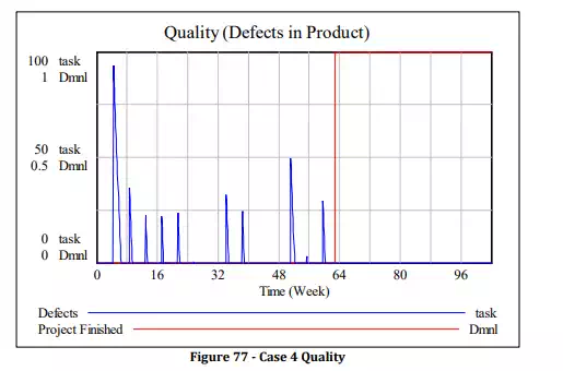
Compared to what we saw in cases 2 and 3, our quality profile shows that defects have a short life on the project, as they are quickly discovered and addressed. This has several positive effects, chiefly: the “Errors upon Errors” dynamic, described in section 4.2, is less powerful, as there are less undiscovered rework tasks dormant in the system at any given time.