Residual analysis is used to assess the appropriateness of a linear regression model by defining residuals and examining the residual plot graphs.

Residual

Residual(ee) refers to the difference between observed value(yy) vs predicted value (y^y^). Every data point have one residual.

residual=observedValue−predictedValuee=y−y^residual=observedValue−predictedValuee=y−y^

Residual Plot

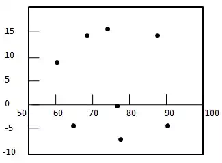
A residual plot is a graph in which residuals are on tthe vertical axis and the independent variable is on the horizontal axis. If the dots are randomly dispersed around the horizontal axis then a linear regression model is appropriate for the data; otherwise, choose a non-linear model.

Types of Residual Plot

Following example shows few patterns in residual plots.

In first case, dots are randomly dispersed. So linear regression model is preferred. In Second and third case, dots are non-randomly dispersed and suggests that a non-linear regression method is preferred.

Example

Problem Statement:

Check where a linear regression model is appropriate for the following data.

xx	60	70	80	85	95
yy (Actual Value)	70	65	70	95	85
y^y^ (Predicted Value)	65.411	71.849	78.288	81.507	87.945

Solution:

Step 1: Compute residuals for each data point.

xx	60	70	80	85	95
yy (Actual Value)	70	65	70	95	85
y^y^ (Predicted Value)	65.411	71.849	78.288	81.507	87.945
ee (Residual)	4.589	-6.849	-8.288	13.493	-2.945

Step 2: – Draw the residual plot graph.

Step 3: – Check the randomness of the residuals.

Here residual plot exibits a random pattern – First residual is positive, following two are negative, the fourth one is positive, and the last residual is negative. As pattern is quite random which indicates that a linear regression model is appropriate for the above data.