The occurrence of failures is usually accompanied by some uncertainty. This is due to many factors that we cannot control, and call them therefore random. Similarly, we speak about random events, which can happen or not, depending on random influences. For their prediction, we use the concept of probability and the related methods. However, before these methods will be explained, several words are addressed here to those who have no or little knowledge of this topic. There are also methods that can improve reliability without probability tools, e.g. Failure Mode and Effect Analysis, which will be explained later. Nevertheless, such methods are suitable only in some cases, whereas the formulas based on probability can facilitate the solution of many reliability problems. Because computers can do all the necessary work, the only thing a user of probabilistic methods needs is some understanding of the basic terms and concepts. The following pages will try to help him or her. Probability is a quantitative measure of the possibility that a random event occurs. The simplest definition of probability P is based on the occurrence of an event in a numerous repetition of a trial

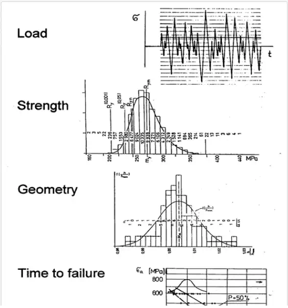
where N is the total number of trials and n is the number of trials with a certain outcome (e.g. a tossed coin with the eagle on the top, the number of days with the maximum temperature higher than 20°C, or the number of defective components). Probability is a dimensionless quantity that can attain values between 0 and 1; zero denotes the impossible event and 1 denotes a certain event. A random variableis a variable that can attain various values with certain probabilities. Random quantities are discrete and continuous. Examples of discrete random quantities are the number of failures during a certain time, number of vehicle collisions, number of customers in a queue or number of their complaints, and number of faulty items in a batch. Continuous random quantities can attain any value (in some interval), such as strength of a material, wind velocity, temperature, diameter, length, weight, time to failure (expressed in hours, kilometers, loading cycles, or worked pieces), duration of a repair, and, also, probability of failure. Examples are depicted in Figure 1. Random quantities can be described by probability distribution or by single numbers, called parameters, if they are related to the population (i.e. the set of all possible members or values of the investigated quantity), or characteristics, if they are calculated from a sample of a limited size. Parameters are usually denoted by Greek letters and characteristics are denoted by Latin letters
Description by parameters
The main parameters (or characteristics) of random quantities are given below, with the formulas for calculation from samples of limited size. Mean μ (or average value) characterizes the position of the quantity on numerical axis; it corresponds to its centroid,

xj is the jth value and n is the size of the sample. The summation is done over all n values.
Variance σ2 (or s2) characterises the dispersion of the quantity, and is calculated as

Standard deviation σ (or s) is defined as the square root of scatter,

It has the same dimension as the investigated variable x, and therefore it is used more often than scatter.
Coefficient of variation ω (or v) characterizes the relative dispersion, compared to the mean value,

It can thus be used for the comparison of random variability of various quantities.
A disadvantage of the average value is its sensitivity to the extreme values; the addition of a very high or very low value can cause its significant change. A less sensitive characteristic of the “mean” of a series of values is median m. This is the value in the middle of the series of data ordered from minimum to maximum (e.g. m = 4 for the series 2, 6, 1, 8, 10, 4, 3).
Description by probability distribution
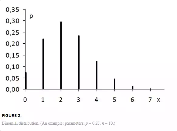
A more comprehensive information is obtained from probability distribution, which informs how a random variable is distributed along the numerical axis. For discrete quantities, probability function p(x) is used (Fig. 2), which expresses the probabilities that the random variable x attains the individual values x*,

Probability density f(x) is used for continuous quantities and shows where this quantity appears more or less often (Fig. 3a). Mathematically, it expresses the probability that the variable x will lie within an infinitesimally narrow interval between x* and x* + dx.
Distribution function F(x) is used for discrete as well as continuous quantities (Fig. 3b) and expresses the probability that the random variable x attains values smaller or equal to x*:

These functions are related mutually as

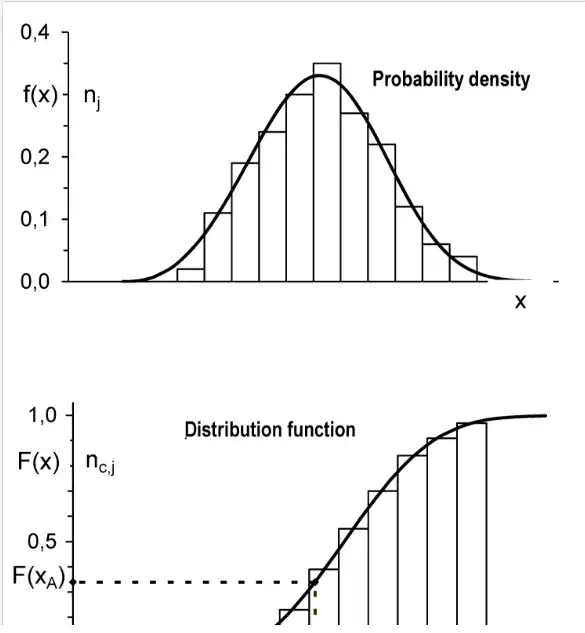
shows two possibilities for depicting these functions: by histograms or by analytical functions. Histograms are obtained by dividing the range of all possible values into several intervals, counting the number of values in each interval and plotting rectangles of heights proportional to these numbers. To make the results more general, the frequencies of occurrence in individual intervals are usually divided by the total number of all events or values. This gives relative frequencies (a) or relative cumulative frequencies (b), which approximately correspond to probabilities.
Fitting such histogram by a continuous analytical function gives the probability density or distribution function (solid curves in Fig. 3). The probability of some event (e.g. snow height x lower than xA) can be determined as the corresponding area below the curve f(x) or, directly, as the value F(xA) of the distribution function. Also very important are the following two quantities.
Quantile is such value of the random quantity x, that the probability of x being smaller (or equal) to is only α,

Quantiles are inverse to the values of distribution function (Fig. 3b),

and are used for the determination of the “guaranteed” or “safe” minimum value of some quantity, such as the minimum expectable strength or time to failure.
Critical value (Fig. 3b) is such value of the random quantity x, that the probability of its exceeding is only β,

The critical values are used for the determination of the expectable maximum value of some quantity, such as wind velocity or maximum height of snow in some area. They are also used for hypotheses testing, for example whether two samples come from the same population. Probability β is complementary to α; β = 1 – α,

More about the basic probability definitions and rules can be found, for example, in [1 – 5].
Probability distributions common in reliability
Several probability distributions exist, which are especially important for reliability evaluation. For discontinuous quantities, it is binomial and Poisson distribution. The main distributions for continuous quantities used in reliability are normal, lognormal, Weibull, and exponential. For some purposes also, uniform distribution, Student’s t-distribution, and chi-square (χ2) distribution are used. The brief descriptions follow; more details can be found in the special literature [1 – 5].
Binomial distribution (Fig. 2) gives the probability of occurrence of x positive outcomes in n trials if this probability in each trial equals p. An example is the number of faulty items in a sample of size n if their proportion in the population is p. The probability function is

and the mean value is μ = np. This distribution is discrete and has only one parameter p, which can be determined from the total number m of positive outcomes in n trials as p = m/n.
Poisson distribution is similar to binomial distribution but is better suitable for rare events with low probabilities p. The probability function giving the probability of occurrence of x positive outcomes in ntrials is

λ is the distribution parameter that corresponds to the average occurrence of x (and, in fact, to the product np of binomial distribution.)
Normal distribution, called also Gauss distribution, resembles a symmetrical bell-shaped curve (Fig. 4). It is used very often for continuous variables, especially if the variations are caused by many random factors and the scatter is not too big (cf. the central limit theorem). The probability density is

with the mean μ and standard deviation σ as parameters. There is no closed-form expression for the distribution function F(x); it must be calculated as the integral of the probability density, cf. Equation (8). In practice, various approximate formulas are also used.
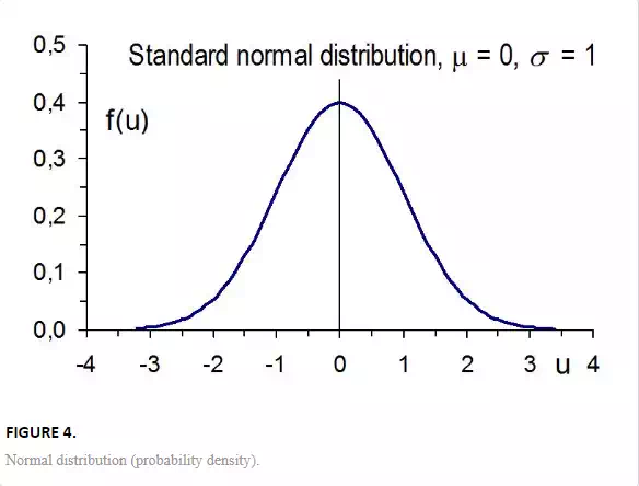
Standard normal distribution corresponds to normal distribution with parameters μ = 0 and σ = 1 (Fig. 4). The expression for probability density is usually written as

u is the standardised variable, related to the variable x of the normal distribution as

It expresses the distance of x from the mean as the multiple of standard deviation. It is useful to remember that 68,27% of all values of normal distribution lie within the interval (μ ± σ), 95,45% within (μ ± 2σ), and 99,73% within (μ ± 3σ).
Log-normal distribution is asymmetrical (elongated towards right, similar to Weibull distribution with β = 2 in Fig. 5) and appears if the logarithm of random variable has normal distribution.
Weibull distribution (Fig. 5) has the distribution function

with three parameters: scale parameter a, shape parameter b, and threshold parameter t0 that corresponds to the minimum possible value of x. The probability density f(x) can be obtained easily as the derivative of distribution function. Weibull distribution is very flexible, thanks to the shape parameter b (Fig. 5). It is often used for the approximation of strength or time to failure. It belongs to the family of extreme value distributions [5, 6] and appears if the failure of the object starts in its weakest part. The determination of parameters of this very important distribution will be explained in Chapter 11.
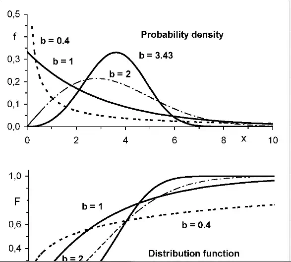
Exponential distribution is a special case of Weibull distribution for shape parameter b = 1, cf. Fig. 5, with the distribution function

which may be used, for example, for the times between failures caused by many various reasons and also in complex systems consisting of many parts. This distribution has only one parameter, T0, which corresponds to the mean μ and has the same value as the standard deviation σ.
The following three distributions are important especially for the determination of confidence intervals, for statistical tests, and for the Monte Carlo simulations, as it will be shown later.
Uniform distribution has constant probability density, f = const, in the interval <a; b>, so that it looks like a rectangle. The mean value is the average of both boundaries, μ = (a + b)/2, and the scatter equals σ2 = (b – a)2/12.
χ2 distribution is a distribution of the sum of n quantities, each defined as the square of standard normal variable. An important parameter is the number of degrees of freedom. For more, see [1–5].
t-distribution (or Student’s distribution) arises from a combination of χ2 and standard normal distribution. It looks similar to normal distribution but also depends on the number of degrees of freedom; see [1–5]. The values of distribution functions and quantiles of the above distributions can be found via special tables or using statistical or universal computer programs, such as Excel. Finally, two important probabilistic concepts should be explained.
Confidence interval. A consequence of random variability of many quantities is that every measurement or calculation gives a different result depending on the used specimen or input value. Thus, the average = Σxj/n is usually determined from several (n) values for obtaining a more definite information. This, however, does not say how far the actual mean μ can be from it. For this reason, confidence interval is often determined, which contains (with high probability) the actual value. For example, the confidence interval for the mean is

and s are the average and standard deviation of the sample of n values, and tα, n-1 is the α– critical value of two-sided t–distribution for n – 1 degrees of freedom. The probability that the true mean μ will lie inside the interval (20), is 1 – α. Confidence intervals can also be determined for other quantities. A note. Also one-sided critical values exist. Such value (α´) corresponds to the probability that the t-value will be either higher or lower than the pertinent critical value. α´ is related to α as α´ = α/2. When using statistical tables or computer tools one must be aware how was the pertinent quantity defined.
Testing of hypotheses. Often, one must decide which of the two products or technologies is better. The decision can be based on the value of the characteristic parameter (e.g. the mean). However, the values of individual candidates usually differ. If the differences are not big, one must consider that a part of the variability of individual values is due to random reasons. Statistical tests can reveal whether the differences between characteristic values of both compared samples are only random or if they reflect a real difference between both types of products. The value of the pertinent test criterion is calculated from basic statistical characteristics of each sample and compared with the critical value (of the probability distribution) of this criterion. If the calculated value is larger than the unlikely low critical value, we conclude that the difference is not random. If it is smaller, we usually conclude that there is no substantial difference between both populations. These tests are explained in the literature [1–5] and available in various statistical or universal programs. Also Excel offers several tests (e.g. for the difference between the mean values or scatters of two populations).
Example 1
The diameters of machined shafts, measured on 10 pieces, were D = 16.02, 15.99, 16.03, 16.00, 15.98, 16.04, 16.00, 16.01, 16.01, and 15.99 mm, respectively. Calculate: (a) the average value and the standard deviation. Assume that the diameters have normal distribution, and calculate (b) the 95% confidence interval for the mean value μD and also (c) the interval, which will contain 95% of all diameters.
Solution
a. The average value is = Σ Di/n = 16.007 mm and standard deviation s = 0.01889 mm.
b. Confidence interval for the mean, calculated by Eq. (20), is (with two-sided critical value t0,05; 10–1 = 2.2622):

The individual values can be expected (under assumption of normal distribution) within the interval – uα/2×s < d < + uα/2×s, where uα/2 is α/2 – critical value of standard normal distribution (corresponding to probability α/2 that the diameter will be larger than the upper limit of the confidence interval, and α/2 that it will be smaller than the lower limit). In our case, u0.025 ≈ 1.96, so that 16.007 – 1.96×0.01889 < D < 16.007 + 1.96×0.01889; that is D ∈ (15.970; 16.044). The reliability of prediction could be increased if tolerance interval were used instead of confidence interval; cf. Chapter 18.


