
A neighborhood café sells out of oat milk every Monday morning, yet throws away pastries on quiet Tuesday afternoons. A retailer fills its warehouse with winter jackets just as temperatures rise. A manufacturer pauses a production line because one low-cost component did not arrive on time.
These are not simply purchasing mistakes. They are demand-and-inventory decisions made under uncertainty. Businesses must decide what customers are likely to buy, when they will buy it, and how much stock should be available before the answer is known.
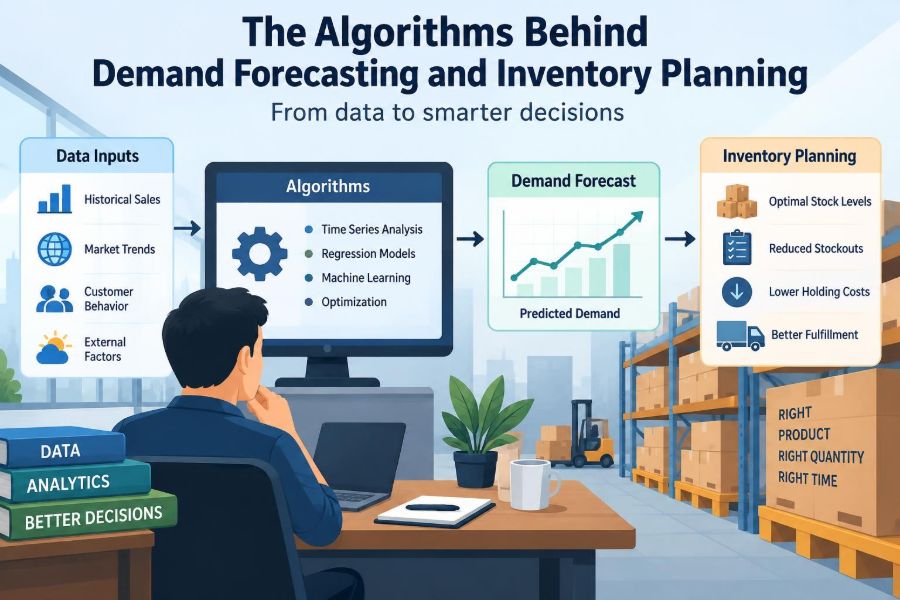
Demand forecasting and inventory planning turn that uncertainty into a structured process. The algorithms involved range from simple averages in a spreadsheet to machine-learning models that combine sales history, prices, weather, promotions, and lead times.
The goal is not to predict the future perfectly. It is to make better trade-offs between having too little inventory, having too much, and tying up cash in the wrong products.
🧭 The Two Decisions at the Heart of Planning
Demand forecasting estimates future customer demand. Inventory planning converts that estimate into decisions about when to order, how much to order, where to place stock, and how much protection to hold against uncertainty.
They are closely connected but not interchangeable. A forecast may say a shop will sell 100 units next month. Inventory planning must still account for current stock, supplier lead time, minimum order quantities, storage constraints, and the cost of a stockout.
A useful forecast with poor replenishment rules can still create empty shelves. Equally, sophisticated ordering software cannot compensate for a forecast that ignores an obvious seasonal pattern.
📦 Why Inventory Is Both an Asset and a Risk
Inventory allows a business to serve customers without waiting for each item to be produced or delivered. It can protect operations from late shipments and smooth the gap between uneven demand and steadier production.
But stock also consumes cash, warehouse space, insurance capacity, and management attention. Perishable goods can spoil; fashion can become outdated; technology can lose value; and slow-moving parts can remain unused for years.
This creates a basic tension: service levels improve when more stock is available, but carrying costs often rise as well. Good planning does not maximize inventory. It aims for an appropriate level of availability at an acceptable cost.
🔍 Start With the Right Definition of Demand
Sales are not always the same as demand. If a product was out of stock, recorded sales may be lower than what customers wanted to buy. If a retailer heavily discounted an item, a spike in sales may reflect the discount rather than normal demand.
Forecasters should also distinguish between customer orders, shipments, returns, cancellations, and internal transfers. Mixing these signals without care can produce misleading patterns.
For example, a distributor that forecasts shipments may need to adjust for a large order that was delayed by credit approval. The shipment occurred this week, but the customer’s underlying need may belong to an earlier period.
🗂️ Build a Reliable Demand History
Algorithms learn from data, so the data must represent the business process being forecast. A practical history usually records product, location, date or week, quantity, price, promotion status, and whether an item was available for sale.
Data cleaning is not an administrative detail. Duplicate orders, incorrect product codes, unit-of-measure changes, and unexplained negative quantities can distort a model more than the choice between two advanced techniques.
Teams should keep a record of data adjustments. If a one-time bulk sale is removed as an outlier, the reason should be visible. Otherwise, a later analyst may unknowingly remove meaningful demand or add the unusual event back into the series.
📈 Recognize Trend, Seasonality, and Random Noise
A demand series usually contains several overlapping forces. A trend is a longer-term movement upward or downward. Seasonality is a repeating pattern, such as higher ice-cream sales in warmer months or greater gifting demand before holidays.
There may also be cycles linked to broader economic conditions, one-off events such as a local festival, and random variation that no model can reliably explain. The planning task is to identify which patterns are stable enough to use.
A rising trend should not automatically be treated as permanent growth. It may reflect a recent promotion, a new customer contract, or a change in product availability elsewhere. Context helps prevent algorithms from extending temporary movements too far into the future.
📏 Choose the Forecasting Granularity Carefully
Forecasts can be made by day, week, month, product, store, customer segment, or region. More detail can make a forecast operationally useful, but it also creates more sparse and volatile data.
A national forecast for bottled water may be fairly stable, while daily forecasts for one flavor in one small store may jump sharply. Aggregating data often reduces noise because variations partly offset one another.
The best level depends on the decision. A factory planning capacity may use a monthly product-family forecast. A fulfillment center allocating stock may require a weekly forecast by location and stock-keeping unit, or SKU.
➗ The Naive Forecast Is a Valuable Baseline
A naive forecast uses a simple rule: next period will equal the most recent period. A seasonal naive forecast says this December will resemble last December, or this Monday will resemble last Monday.
These methods sound basic, yet they are difficult to beat for some stable or highly irregular product lines. They also provide a benchmark: a complex model should demonstrate that it improves decisions beyond a sensible simple rule.
If a machine-learning system performs worse than a seasonal naive forecast in back-testing, adding more technical language will not make it more useful. The team should inspect the data, the model inputs, and the evaluation design.
📊 Moving Averages Smooth Short-Term Variation
A moving average averages demand from a recent set of periods. A three-month moving average, for example, uses the previous three months to forecast the next one.
Because unusually high and low observations are blended together, the method smooths random movement. It works best when demand is relatively stable and there is no strong trend or seasonal pattern.
The window size matters. A longer window gives a calmer forecast but reacts slowly when conditions change. A shorter window responds faster but can chase noise. Selecting it is a business choice as much as a mathematical one.
⚖️ Weighted Averages Give Recent Data More Influence
Not every past observation needs equal weight. A weighted moving average can assign more influence to recent demand and less to older periods.
This is useful when recent sales better represent current conditions, such as after a distribution expansion or a gradual shift in consumer preferences. However, it can overreact to a short-lived event if weights are too concentrated on the latest data.
A manager should be able to explain why the weighting scheme fits the product’s behavior. Arbitrary weights may create an appearance of precision without a sound operational reason.
📉 Exponential Smoothing Learns as New Data Arrives
Exponential smoothing updates a forecast each time new demand is observed. It gives greater weight to recent periods while retaining information from earlier periods in a declining pattern.
Simple exponential smoothing is suited to demand with no clear trend or seasonality. Extensions can explicitly model a trend and recurring seasonal effects, making the family of methods flexible for many business settings.
The smoothing parameters control responsiveness. High responsiveness can detect genuine shifts sooner but may turn routine fluctuation into unnecessary purchase orders. Lower responsiveness produces steadier plans but may lag behind a real change.
🧮 Regression Connects Demand to Its Drivers
Regression models estimate the relationship between demand and possible explanatory variables. These may include price, promotional activity, day of week, store characteristics, weather indicators, or a marketing campaign.
For instance, a retailer might model demand for umbrellas using rainfall forecasts, season, and price. The model does not claim rain alone causes every sale; it estimates how demand has tended to move when relevant conditions occurred together in past data.
Regression requires caution. A variable that moves alongside sales is not automatically a usable cause. Promotions are often scheduled when managers already expect high demand, which can make their apparent effect difficult to separate from the underlying pattern.
🧠 Machine Learning Finds Complex Patterns
Machine-learning algorithms can combine many inputs and capture nonlinear relationships, such as a discount having a different effect during a holiday period than during an ordinary week. Common approaches include tree-based models, neural networks, and ensembles that combine several models.
They can be useful for large catalogs and many locations, especially when external signals are meaningful and available ahead of time. Yet more complexity introduces risks: hidden bias in inputs, harder explanations, greater maintenance needs, and overfitting.
Overfitting occurs when a model learns accidental details of historical data rather than patterns likely to recur. It can look impressive during development and fail when faced with new conditions.
🧪 Test Models on the Future, Not the Past
A forecasting model should be evaluated by training it on earlier periods and testing it on later periods that were not used to build it. This reflects the real planning problem: making a decision before demand is known.
For time series, data should not be randomly shuffled in the usual way. Doing so can let information from the future leak into the past. Instead, teams commonly use rolling evaluations, repeatedly moving the forecast origin forward through time.
Testing should mirror the operational forecast horizon. A model that predicts one week ahead well may not be appropriate for a supplier whose lead time requires a twelve-week ordering decision.
🎯 Measure Error in a Business-Relevant Way
Forecast accuracy measures compare predictions with actual outcomes. Absolute error shows the size of misses, while squared-error measures penalize large misses more heavily. Percentage-based measures can be useful but become unstable when actual demand is near zero.
No single metric suits every catalog. A one-unit error on an expensive aircraft component and a one-unit error on a low-cost pen do not have the same consequence.
| Measure | Useful when | Key limitation |
|---|---|---|
| Absolute error | Comparing error in actual units | Hard to compare products with very different volumes |
| Percentage error | Comparing scale across many products | Can mislead when actual demand is zero or very low |
| Bias | Detecting consistent over- or under-forecasting | Positive and negative errors can cancel out |
| Service impact | Linking forecasts to availability and stockouts | Also depends on lead time and inventory policy |
Forecast bias deserves special attention. A model that is repeatedly low may cause stockouts even if its average absolute error appears acceptable. A consistently high forecast can quietly create excess inventory.
🪜 Translate Forecasts Into Replenishment Decisions
Once demand is forecast, inventory rules determine the response. A common approach sets a reorder point: when inventory position falls to a specified level, the business places an order.
Inventory position usually includes stock on hand plus stock already ordered, minus committed demand. The reorder point should cover expected demand during the supplier lead time plus a buffer for uncertainty.
For example, if a component normally sells at 20 units per week and takes three weeks to arrive, expected lead-time demand is roughly 60 units. The company may hold additional safety stock if demand or delivery timing varies.
🛡️ Safety Stock Protects Against Uncertainty
Safety stock is extra inventory held to reduce the risk of running out when actual demand exceeds expectations or replenishment arrives late. It is not a substitute for poor data or unreliable suppliers, but it can absorb normal variation.
The appropriate buffer depends on demand variability, lead-time variability, desired service level, and the consequences of a stockout. A missed sale may be minor for a replaceable office item but costly for a critical production part.
Too little safety stock creates frequent expedites and disappointed customers. Too much masks process problems and raises holding costs. The right level should be reviewed as demand patterns and supplier performance change.
🚚 Lead Time Is More Than Shipping Time
Lead time begins when a replenishment decision is made and ends when usable inventory is available. It can include approval delays, supplier processing, production, transportation, receiving, quality inspection, and put-away.
Using an optimistic shipping estimate while ignoring the rest of the process understates the inventory needed. Lead time also varies: a supplier that usually delivers in two weeks but occasionally takes five creates more uncertainty than a consistently three-week supplier.
Reducing lead-time variability can sometimes lower inventory more effectively than making a small improvement to forecast accuracy. Operations, procurement, and suppliers therefore all influence inventory performance.
📐 Order Quantity Balances Competing Costs
Replenishment involves not only timing but quantity. Ordering very frequently can increase administrative, transport, setup, or receiving costs. Ordering large batches can raise storage costs and the risk of obsolescence.
The classic economic order quantity model balances ordering cost against holding cost under simplified assumptions. It can offer a useful starting point, but real operations may face quantity discounts, capacity limits, seasonal demand, short shelf life, and supplier minimums.
Algorithms should support judgment rather than force a mathematically tidy order size into an impractical warehouse or cash-flow position.
🧩 Segment Products Before Applying One Rule to All
Not every SKU deserves the same forecasting effort or inventory policy. ABC analysis groups items by their relative business impact, often based on annual consumption value. A small number of high-value items may require closer control than a long tail of inexpensive items.
Demand behavior matters too. Stable, high-volume products suit different methods from intermittent spare parts or short-life seasonal goods.
- High-value, stable items: frequent review and carefully tuned replenishment rules.
- Low-value, stable items: simpler controls may be sufficient.
- Intermittent items: specialized methods, shared stock, or make-to-order policies may be better.
- Seasonal items: early commitment decisions and end-of-season markdown planning become central.
Segmentation directs analytical effort where it changes outcomes most.
🌦️ Treat Seasonal Products as a Distinct Planning Problem
Seasonal inventory often has a limited selling window. A business cannot simply replenish after demand is observed if the supplier lead time extends beyond the season.
For these products, planners combine prior seasons, pre-orders, market information, and scenario ranges. They must also consider the cost of leftover stock, including clearance discounts, storage, and disposal.
A hypothetical swimwear retailer may order more cautiously when styles are highly trend-sensitive and leftovers have little value. It may order more aggressively for basic items that can be sold in a later season.
🕳️ Handle Intermittent and Lumpy Demand Differently
Intermittent demand contains many periods with zero sales, followed by occasional purchases. Replacement parts, specialized industrial supplies, and certain medical or maintenance items often behave this way.
A normal average can be misleading because it hides two separate questions: how often will demand occur, and how large will it be when it occurs? Methods designed for intermittent demand estimate occurrence and size separately.
Even then, uncertainty remains high. Businesses may need to use service agreements, repairable-item pools, substitute parts, or central stocking rather than relying solely on a point forecast.
🔗 Use External Signals Only When They Are Available in Time
Weather, search activity, event calendars, economic indicators, and promotional plans can improve forecasts when they are relevant and known before the ordering decision. The timing condition is crucial.
A store cannot use next week’s realized weather to order inventory today, but it may use a weather forecast. Similarly, a campaign calendar can be useful if marketing confirms the plan early enough for supply decisions.
External inputs should be monitored for quality. A changed promotion plan or unreliable data feed can harm a model that has become dependent on that signal.
🤝 Combine Statistical Forecasts With Business Knowledge
Statistical models excel at consistently processing history. Sales teams, product managers, and operations staff may know about a new contract, competitor exit, packaging change, or planned campaign that history cannot reveal.
A structured forecast review can combine both strengths. The statistical forecast provides a starting point; business users propose adjustments with a documented reason, estimated effect, and owner.
Unexplained overrides should be avoided. If managers routinely replace the model with intuition, the organization loses the ability to learn whether those adjustments improved accuracy or merely reflected confidence.
🔄 Sales and Operations Planning Aligns Assumptions
Demand planning affects purchasing, production, finance, staffing, transport, and customer commitments. Sales and operations planning creates a regular process for agreeing on a feasible demand-and-supply view.
The conversation should focus on assumptions and choices, not just a single forecast number. What happens if demand is stronger than expected? Which products receive priority if capacity is constrained? How much inventory can the business afford to carry?
Scenario planning makes uncertainty visible. A base case, upside case, and downside case can reveal where flexibility is needed before a shortage or surplus becomes urgent.
🏬 Plan Across a Network, Not Just One Warehouse
Businesses with multiple stores, warehouses, or distribution channels must decide where inventory should sit. Holding some stock centrally can pool risk because demand peaks in one location may be offset by quieter demand elsewhere.
Decentralized stock can improve delivery speed and local availability, but it may duplicate buffers across sites. The appropriate design depends on transport speed, service promises, product size, demand variability, and transfer capability.
Algorithms can recommend allocation, but the result must respect physical constraints such as dock capacity, storage space, and route schedules.
⚠️ Watch for the Bullwhip Effect
The bullwhip effect occurs when small changes in customer demand create larger swings in orders upstream. A retailer sees a modest increase, orders extra to protect stock, and the wholesaler interprets the larger order as a major demand surge.
Long lead times, batch ordering, price promotions, shortage gaming, and poor information sharing can amplify the effect. Manufacturers then may build too much capacity or inventory based on distorted orders.
Sharing point-of-sale demand, reducing unnecessary order batching, and using stable replenishment rules can reduce this amplification. The aim is to react to actual consumption rather than every fluctuation in replenishment orders.
🧾 Understand the Limits of Automation
Automated planning systems can process thousands of items more consistently than manual spreadsheets. They can flag exceptions, refresh forecasts, and calculate suggested orders quickly.
However, automation cannot decide whether source data is trustworthy, whether a new product is comparable to an older one, or whether a proposed order fits a strategic decision. It may also repeat errors at scale if settings are wrong.
Good governance includes clear ownership of master data, approval rules for unusually large orders, audit trails, and regular checks of model performance. Human review should focus on material exceptions rather than routine transactions.
🧱 Avoid Common Forecasting and Inventory Mistakes
- Using sales as unquestioned demand: stockouts and lost sales can hide real customer interest.
- Choosing the fanciest model first: a strong baseline and clean data usually matter more.
- Forecasting at an unusable level: a national monthly forecast may not support local daily replenishment.
- Ignoring lead-time variation: average lead time alone can produce understocking.
- Measuring accuracy but not bias: consistent under-forecasting may remain invisible.
- Applying identical rules to every SKU: stable staples and rare spare parts need different policies.
- Failing to learn from overrides: undocumented judgment cannot be evaluated or improved.
Many of these failures are process failures rather than mathematical failures. Better model design cannot fully repair fragmented data ownership or incentives that reward one department at another’s expense.
🛠️ Build Capability in Practical Stages
Organizations do not need to begin with a large artificial-intelligence program. A sensible first step is to define the decision, create a clean demand history, establish a simple baseline, and measure results over time.
Next, segment the catalog and improve the areas with the largest operational impact. This may mean better lead-time records for critical components, seasonal planning for a limited product group, or formal review of promotional forecasts.
Only then should teams add complexity where evidence supports it. A more advanced model is worthwhile when it improves service, reduces avoidable stock, or helps planners make decisions that simpler methods cannot support.
🧭 The Core Principle: Decisions Under Uncertainty
Demand forecasting is not a contest to produce the most impressive prediction. Inventory planning is not a race to hold the least stock. Both are disciplines for making explicit, repeatable decisions when future demand and supply conditions are uncertain.
The strongest systems connect good data, an appropriately simple model, realistic lead times, product-specific policies, and regular business review. They measure not only forecast error, but also stock availability, excess inventory, bias, and the cost of exceptions.
When forecasts are treated as informed estimates rather than certainties, teams can plan buffers, scenarios, and response options with much greater discipline.
The practical advantage comes from matching the algorithm, the inventory rule, and the business context—not from relying on any single formula to predict an unpredictable future. With that foundation, better availability and healthier inventory levels become achievable planning outcomes rather than hopeful guesses. 📊📦